Make the most of your GPU

The last couple of weeks, I have been playing around with data from my favorite app, iNaturalist. The good folks there, have released a dataset with 2.6M images of 10,000 species of assorted beasts and other flora. I’ve been trying to build a model that can separate the Jungle Babbler from the Yellow-Billed Babbler, a task that would be beyond most non-ornithologically minded humans.

1. Data Flow when Training on a GPU
2. The Metric 
3. The hardware
4. Data Loader Throughput 
5. Model Training Throughput
   1. Batch Size
   2. Mixed precision 
   3. Memory Pinning 
6. Turning Some Knobs
   1. Mixed Precision
   2. Num Workers in Data Loader
7. Don’t waste time and money optimizing the wrong part of your pipeline
8. Some Questions to chew on 
9. What if we use two T4 GPUs
10. What if we use a high end GPU like the V100
11. Closing Thoughts 
12. Further Reading
13. Update on Training with a V100

Training Deep learning models on your own dime on the cloud can quickly make the costs of Deep learning a very concrete concept. Without the privilege of a GPU cluster, bankrolled by your tech overlords, what’s an independent engineer gotta do ?

In this post we will look at getting the most bang from a single mid end GPU on the google cloud. 

Data Flow when Training on a GPU

Let us start from first principles and take a look at how data flows when you train on the GPU. 

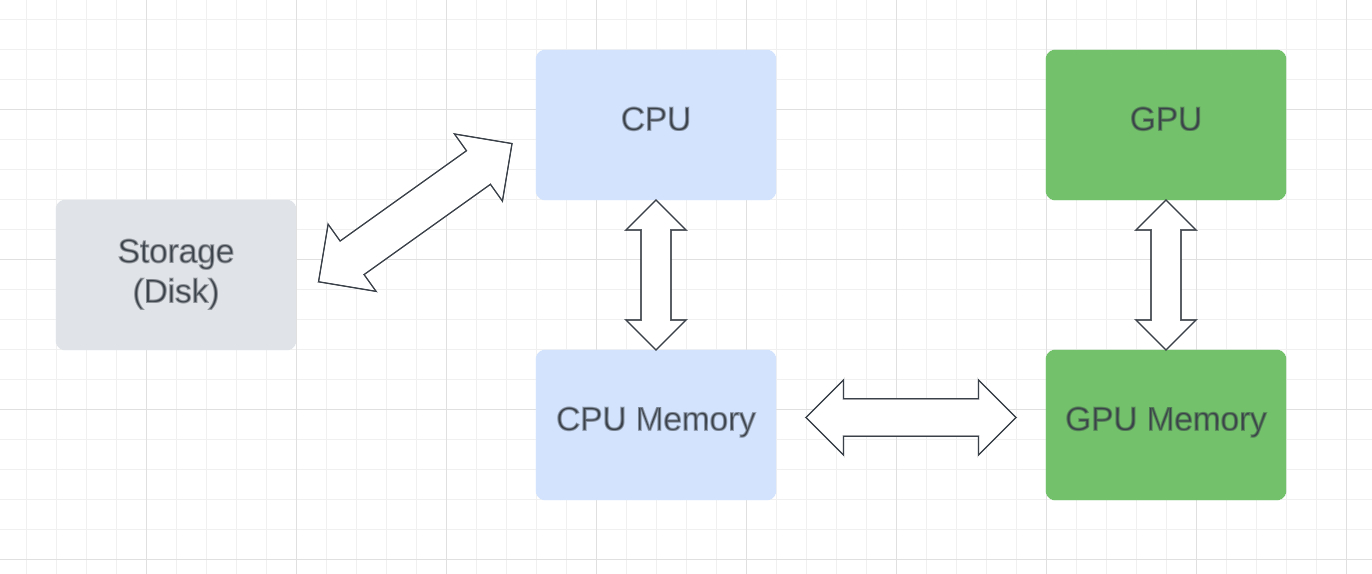
Roughly we can separate out three stages 

1. The CPU reads data from Disk and puts it on CPU memory (RAM in common parlance)
2. Data is copied from CPU memory to GPU memory
3. The GPU runs on data on the GPU memory 

Like a plumbing system with pipes of different diameters, the overall flow is determined by the  narrowest pipe. You don’t want mismatched pipes where data back ups and bad things happen (OOM errors) or your most expensive pipe (the GPU) running empty.  

The Metric 

Of course we want to build the best model very fast. Metrics for model quality are typical ML metrics like accuracy. For speed, at first time taken (for 1 epoch ) can seem like a reasonable choice, but it is not. It does not allow us to easily measure speeds in Stages 1 and 2 in the figure and also is obviously dependent on dataset size, making comparisons impossible. 

Instead we will measure throughput or samples processed per second. Since we are dealing with images this is images per second in our example. This is a great metric that directly relates to how long training takes and can be compared across different tasks, bringing out bottlenecks in our data flow. 

The secondary metrics which we will also track and use for diagnostics are 

1. GPU Utilization, which measures how busy the GPU is. More the better.
2. GPU memory usage ,which measures how close we are to getting an OOM error on the GPU. We should aim to be around 80% 

The hardware

I ran everything on the Google Cloud and used a VM with these specs.

1. 4 vCPUs with 32 GB RAM (N1 series in GCP jargon)
2. 1 NVIDIA T4 GPU with 16GB memory . This is the so-called commoners GPU and is about 7X cheaper per hour than the fancy V100. NVIDIA recommends this for inference workloads although it’s a reasonable choice for training. Importantly it supports mixed precision operations (More on this later)
3. For storage, I used a balanced persistent disk (in GCP jargon). This is basically an SSD, but not on the same board as the CPU. I was very curious to see if this would be a bottleneck as network calls are involved in fetching data (Ans: It wasn’t) 

Data Loader Throughput 

We start off by measuring throughput of just loading the data from disk. This gives us an upper bound for achievable throughput. I often see folks not measuring this and wasting time optimizing the wrong thing. If your GPU throughput is lower than the Data Loader throughput, there is no point in optimizing the Data Loader stage.

Here is some PyTorch code that creates a Dataset, wraps it around a DataLoader and measures images processed per second. 

We vary the number of worker processes dedicated to reading data and run through a few hundred batches to see what throughput looks like.

We see that throughput starts plateauing at about 4 workers. I was curious to see if the “balanced persistent” disks that GCP has were slowing things down. I ran the same experiment on my MacBook

So, with 1 worker, DataLoading is indeed faster with the MacBook’s SSDs, but increasing the number of worker processes makes reading data from GCP’s network mounted disks, roughly as fast as reading from a locally mounted SSD. Note that increasing the number of workers increases the RAM usage as each process maintains its own copy of objects.

Model Training Throughput

Here are some knobs that folks usually tune to optimize model training throughput. We will go over them briefly. 

Batch Size

This is the number of samples inside the batch that gets sent to the GPU during the forward pass. GPU’s have multiple tensor cores that are optimized for matrix operations and can perform the forward pass on an entire batch in one go, by utilizing these cores in parallel.  This is obviously faster than performing the forward pass for one sample at a time.  I see a lot of folks advise increasing batch size as the first lever to pull to make training faster. I don’t agree for two reasons

1. Large batch sizes make training neural nets more finicky. There is a lot written about poor model accuracy when training on large batches. Smaller batches have a regularization effect as the “noisy” weight updates of SGD help it settle to a better minima. See this paper for more details. 
2. Increased batch sizes will only increase throughput if the GPU is currently under utilized. Also increasing batch sizes increases GPU memory being used and limits the size of the model (that is also on the GPU memory) that you can create.

Mixed precision 

Modern GPUs and TPUs have  tensor cores that can do floating point operations much faster in 16 bit as compared to 32 bit. The memory used is lower too, allowing for larger models to be trained. The downside is that with the lower range for float 16, numerical problems like underflow or overflow can pop up. Frameworks like PyTorch and Tensorflow offer Mixed precision, which automagically cast some parts of the network to float16 and use float32 only on ops deemed to need the extra numerical range. An important detail we need to  keep in mind is that the gradient for ops that use float16, could underflow to zero , so we scale them higher before doing the backward pass. DL Frameworks, handle all this for you, conveniently wrapping the optimizer in a GradScaler.

Memory Pinning 

This speeds up data transfer from CPU memory to GPU memory, by using a block of non pageable memory called “Pinned memory” inside the CPU’s RAM to stage the transfer. You can think of this block as a dedicated buffer that is not de-allocated during the data loading pipeline. 

Turning Some Knobs

Now that we have a handle on the knobs,  it’s time to plug in our model and measure throughput as we turn these knobs. . I used a resnet50 model , where the last Fully connected Linear layer is replaced with one with 10,000 output features (we have 10,000 classes in the iNaturalist dataset).

To profile throughput, I just plotted metrics on Tensorboard. The primary metric we care about is Images processed per second. We will also look at GPU utilization and GPU memory usage. All this stuff is easy to access inside your training code and we don’t need to use a special profiler to do this. I recommend this simple profiling first, and only then using the PyTorch profiler, which provides deeper visibility.

This is how the throughput curves look like. On the y-axis we have Images processed per second and on the x-axis is the batch index. Each line represents a particular configuration. For example one of the lines in the middle cluster (having throughput ~ 160 ) is BATCH_SIZE=32;NUM_WORKERS=1;USE_AMP=True;PIN_MEMORY=True. 

Also note how the throughput curves take time to warm up. This is expected. 

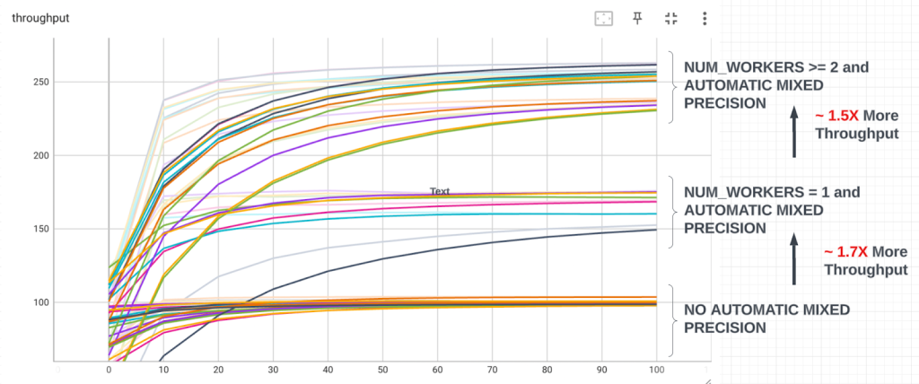
Plotting the throughput like this, the curves quite neatly cluster into 3 groups and the insights scream out

1. Enabling mixed precision makes a huge difference and provides  ~ 1.7X more throughput
2. Using 2 or more workers in the Data Loader also makes a huge difference , providing ~ 1.5X more throughput
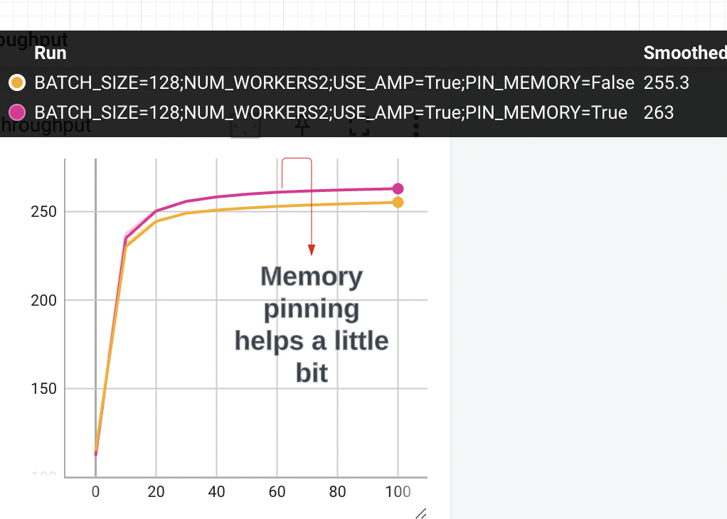
3. The highest throughput is around ~260 Images per second for this config BATCH_SIZE=128;NUM_WORKERS=2;USE_AMP=True;PIN_MEMORY=True

Memory Pinning also helps, but only provides modest gains in throughput. Here is a cleaned up graph where we fix batch size, num workers and use automatic mixed precision 

Let’s dig a bit deeper into the knobs that mattered the most

Mixed Precision

We saw enabling this gave us the largest boost (~1.7X more throughput), but how does it affect GPU utilization? Lets clean up the graph and use a fixed batch size of 128 and 2 workers in data loader 

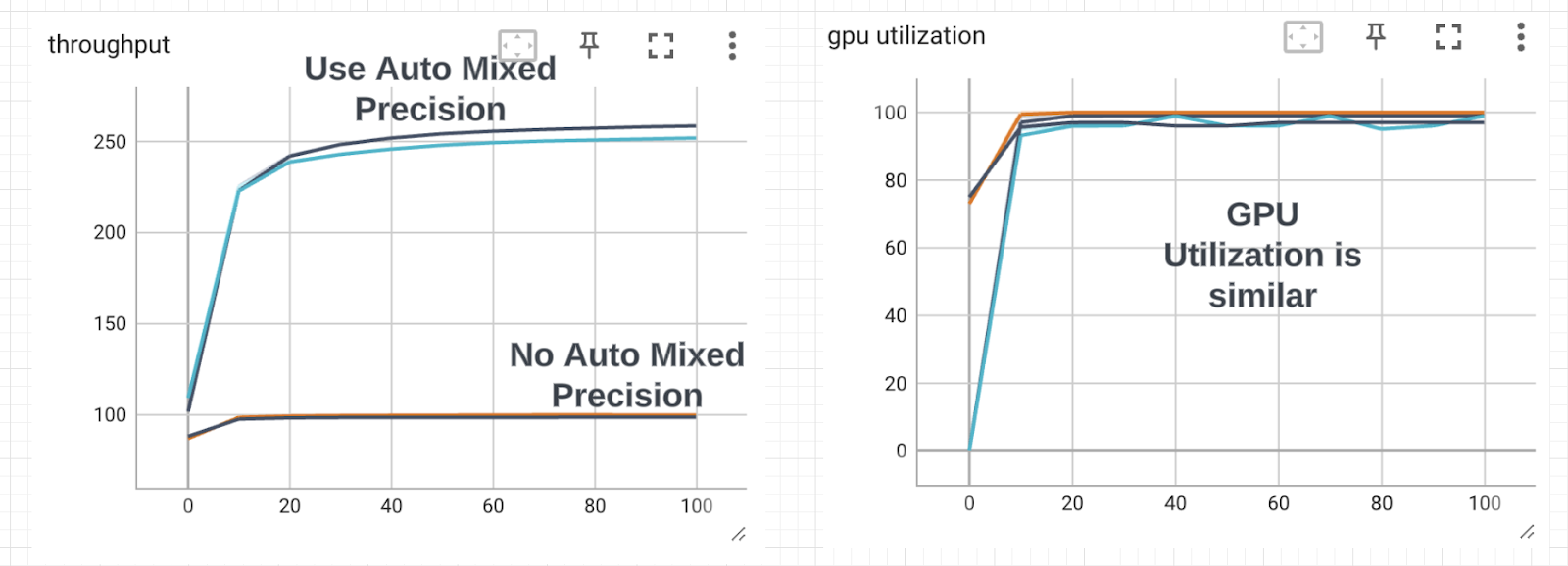
The lesson here is that  looking only at GPU utilization can fool us into thinking that we cannot increase throughput. By using Automatic mixed precision, we are able to do many more ops per second and that translates to the increased throughput

Num Workers in Data Loader

Why do we see a step change in throughput when we use more than 2 workers in the Data Loader. The graph in the figure are using batch size of 128, fixing the number of workers to 1 and enabling automatic mixed precision.  

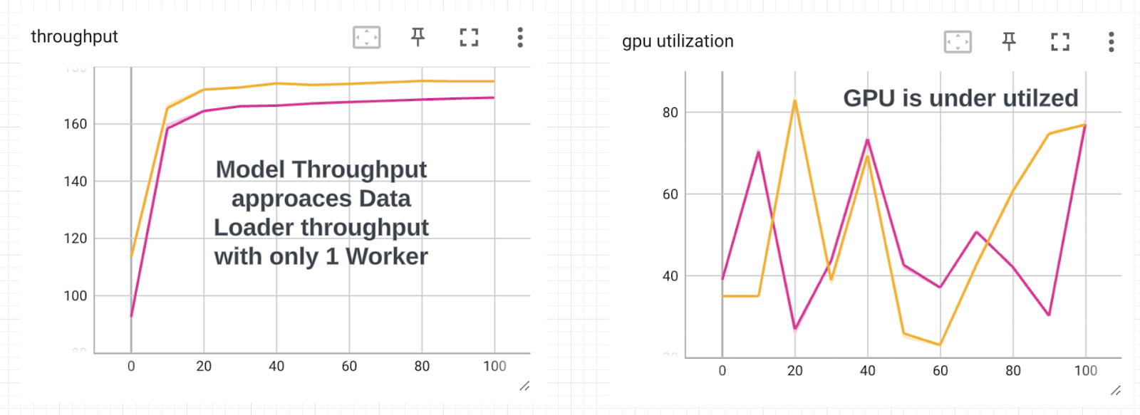
The model throughput approaches the Data Loader throughput with 1 worker and the GPU utilization is lower.  This means that when we use less than 2 workers, the bottleneck is the Data Loading stage. The GPU is sitting idle waiting for more tensors to crunch. 

Don’t waste time and money optimizing the wrong part of your pipeline

Now that we understand the whole pipeline at a deeper level, we can go beyond just tuning knobs blindly and hoping for the best. 

For this particular setting of hardware, it would be a waste of time trying these things

1. Paying more for faster SSD’s that are directly attached to the VM
2. Trying to do any pre-processing for images offline. For example you might think that doing image resizing and scaling beforehand might be helpful. It won’t since we are easily able to achieve higher data loader throughput than what the GPU can handle (when we use more than 1 worker)
3. Using more than 2 workers for Data Loading is pointless and can lead to Out Of Memory errors . 
4. Paying for more vCPU’s or CPU RAM would be wasted money 
5. Increasing batch size beyond 128, does not help throughput and could potentially give you a bad model. In fact using a batch size of 64 (with Auto Mixed precision, 2 worker threads and memory pinning) is probably a better choice than using a batch size of 128 as it gives similar throughput. See earlier notes on batch size and model regularization.

Some Questions to chew on 

After running these experiments to measure throughput, the obvious next question is how can we increase throughput  beyond the 260 Images per second we were able to get to. 

Since we are GPU compute bound, the answer lies in getting more GPU compute. 

But this gets interesting. Should we get one more T4 GPU and run distributed training with multiple GPUs or go for a higher end single GPU like the V100. I haven’t run any experiments to answer this question fully, but we can still take an informed guess.

What if we use two T4 GPUs

Keeping everything else the same and using a Distributed Data Parallel model training strategy  , we should expect slightly less than 2X  increase in throughput if we add another T4. The reason is that the Data Loader throughput with 4 workers is around ~440 and using 2 T4’s GPUs we get to ~ 520 Images per second (I just assumed 2X of the 260 Images/sec we got with 1 T4). 

To utilize both the GPU’s we would need to increase vCPUs and RAM on the GCP VM. Another thing to be aware of is that using multiple GPUs would lead to increased overhead since the weight updates have to be synchronized across GPUs, so we should expect maximum achievable utilization to drop a bit when we add more GPU’s.  

What if we use a high end GPU like the V100

The V100 claims to deliver over 100 Tensor TFLOPS (1 TFLOP = 10^12 tensor ops per second) and is around 7X more expensive to run than the T4 which has around 8 TFLOPS (using fp32) . Will 1 V100 be 7 times as fast as a single T4 ?

To answer this question, I took a look at the V100 datasheet. The claim is that the V100 offers 32X speedup over a CPU in training a resnet50  model. Somewhere in the footnotes, they mention that the CPU throughput is 48 Images per second.

So 32X of that gives us = 32 X 48 = 1536 Images per sec. 

On 1 T4 we got to 260 Images per sec. So, 7X of 260 should have been 1820 Images per sec.

So if we spend 7X more (and increase CPUs and RAM to keep up) , my guesstimate is that we get  around 6X (1536 Images per sec)more throughput. 

[Edit – This turned out to be wrong]

It makes sense to me that GCP pricing would be structured this way. 

The most expensive component in any DL pipeline is the human in the middle, and using a faster and more expensive GPU means lesser time spent waiting for the model to train. It doesn’t matter that the performance scales sub linearly with the price and GCP (which is fully aware of this) charges more for lesser bang.

Closing Thoughts 

In this post, we took a look at how to increase model throughput by understanding the data loading and model training pipeline. It’s trivial to instrument your training code to track throughput. Before training your model for several epochs with whatever default parameter PyTorch uses, it pays to run a few experiments to understand where the bottleneck is.

In summary I would recommend this sequence in optimizing training throughput

1. Measure throughput of just Data Loading
2. Use Automatic Mixed Precision. This will almost always increase model throughput, There is an odd chance of loss exploding, but this risk is tiny for well known model architectures like Resnet, et al
3. Set the number of workers in the Data Loader to the minimum required to unblock the GPU. Using more workers than necessary will result in OOM errors
4. Use the minimum batch size that takes you close to the max achievable throughput. Using unnecessarily large batch sizes will likely lead to a poorer model and limits the size of the model you can train.
5. Use memory pinning
6. Marry the right CPU/RAM to the GPU. 

As with everything in Deep Learning, all these recommendations are probably tied up to the model architecture. Understanding the pipeline from first principles is the only way to avoid frustrations of blindly tuning knobs and blowing your costs.

Further Reading

1. Paper on how batch size can affect model accuracy
2. Automatic Mixed Precision explained by NVIDIA
3. Automatic Mixed Precision tutorial by PyTorch
4. Memory Pinning explained by NVIDIA
5. NVIDIA T4 Data sheet

Update on Training with a V100

I was really curious to see how using a V100 would speed things up. I increased vCPU to 12 (GCP strangely limits this) and looked at throughput. For simplicity, I am plotting only configs with Auto Mixed precision enabled and with Pinned memory. I used way more workers in the Data Loader.

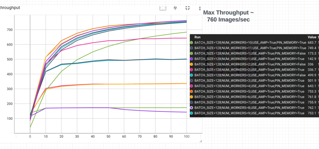
Frankly, I was underwhelmed. We get to 760 Images per sec, which is about 3X of what I was seeing on the T4. I made sure that GPU utilization was close to 100% (it was). So paying 7X more only gives us 3X more throughput .

I looked more closely at the V100 Data sheet, and noticed that they used MxNet , instead of PyTorch. Also the hardware is a V100 with 32 GB GPU memory. Could these differences explain the gap ? Interestingly MxNet claims that in an NVIDIA benchmark they came out 77% faster on resnet.

Either way, our guesstimate that throughput scales sub-linearly with price seems directionally correct, but needs a bit of downward adjustment. GCP sure knows that engineer time is orders of magnitude more expensive than GPUs